Neural Networks are some of the weirdest tools created and can be used for image recognition, optimal control solution, or motion prediction. Being interested in them for the longest time motivated me to try and utilize them for a project.
Motivation
Starting this project came from wanting to learning more constructing neural networks; I’ve always watched those videos such as 3Blue1Brown’s series on neural networks.
Watching these videos are great to learn, but just like reading from an engineering textbook, its a little useless you do the practice problems in the back of the book. So, wanting to create something using neural networks, I needed to find the problem I wanted to solve. Being interested in dynamics, I chose a pendulum problem to motivate the work.
The pendulum problem is defined as known time series solution for the path a pendulum will take as it swings given a initial conditions. Being one of the classical examples for explaining numerical methods and implementing solutions like the small angle assumption or using forward Euler integration. Since I have been exposed to these classical examples in my undergrad constantly, I wanted to see if I could solve this problem using a neural network.
Choosing the Right Model
The effectiveness of a neural network is completely dependent on the type of model chosen for the problem. Many varieties of the neural network exists, such as convolutional or recurrent networks. Determining what network is best depends on the use case. For the convolutional neural network, learn-able biases and weights are given to the neurons initially, and are typically given large matrices as inputs, making them great for image recognition. For the recurrent neural network, the feedback of the output of a layer is used in the input again. This principle helps to predict the outcome of the layer, with each neuron acting as a memory cell, retaining some information as it goes to the next time step. This process is especially helpful in motion prediction, which is the what the pendulum problem is trying to solve!
Solving the Pendulum Problem Numerically
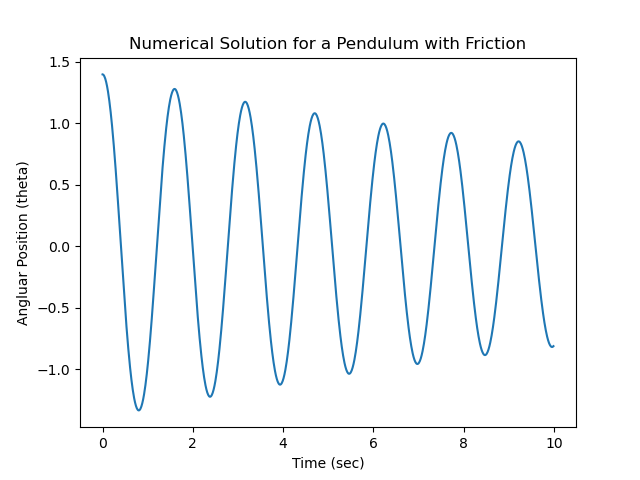
In order to correctly train the recurrent neural network (RNN), the numerical solution was needed to ensure the model was output the correct data. Below, I placed the main Python script I used to find the solution for the pendulum problem. Note both the friction and non-friction versions of the equations are defined if you wanted to see the difference to the two types of equation sets.
import numpy as np
import matplotlib.pyplot as plt
from scipy import integrate
import math

L = 0.5
g = 9.81

b = 0.1
m = 1


def pendulumODE(theta,t):
    dtheta1 = theta[1]
    dtheta2 = -g/L*math.sin(theta[0])
    return [dtheta1, dtheta2]

def pendulumODEFriction(theta,t):
    dtheta1 = theta[1]
    dtheta2 = -b/m*theta[1]-g/L*math.sin(theta[0])
    return [dtheta1, dtheta2]

t0,tf = 0,10
t = np.arange(t0, tf, 0.01)

theta0 = [(math.pi/180) * 80, (math.pi/180) * 0]

r = integrate.odeint(pendulumODEFriction, theta0, t)
# LSODA is the closest integrator to ODE45 in matlab

plt.plot(t,r[:,0])
plt.xlabel("Time (sec)")
plt.ylabel("Angular Position (theta)")
plt.title("Numerical Solution for a Pendulum with Friction")
plt.show()
Hyperparameters and Initial Conditions
Now that the pendulum problem has been solved numerically, we can begin applying the RNN to the problem. To begin, a data set is needed to train the RNN; this was easily generated using the code snippet below, where 100 data sets were randomly generated based on a random generation of initial conditions for the problem. Here, I chose a pretty narrow range for the initial conditions, with an position IC of 70-90 degrees always constrained to 0 initial velocity. Doing so drastically improved my model due to overfitting; in the future I want to expand the range (but I’ll touch on this later).
DATA_SET_SIZE = 100
# initilize the arrays used to store the info from the numerical solution
theta = [0 for i in range(DATA_SET_SIZE)]
numericResult = [0 for i in range(DATA_SET_SIZE)]
output_seq = [0 for i in range(DATA_SET_SIZE)]
# generate random data set of input thetas and output thetas and theta dots over a time series
for i in range(DATA_SET_SIZE):
    theta = [(math.pi/180) * random.randint(70,90), (math.pi/180) * 0]
    # numericResult[i] = integrate.solve_ivp(pendulumODEFriction, (t0, tf), theta, "LSODA")
    numericResult = integrate.odeint(pendulumODEFriction, theta, t)
    output_seq[i] = numericResult[:,0]
    if i == DATA_SET_SIZE-1:
        actualResultFull = integrate.odeint(pendulumODEFriction, theta, np.arange(t0, 2*tf, TIME_STEP))
        actualResult = actualResultFull[:, 0]
Once the data set was generated, an elementary(for neural networks) RNN was constructed. This class follows the default class constructed using the PyTorch example.
class pendulumRNN(nn.Module):

    def __init__(self, hidden_dim):
        super(pendulumRNN, self).__init__()

        self.hidden_dim = hidden_dim

        self.lstm1 = nn.LSTMCell(1,self.hidden_dim)
        self.lstm2 = nn.LSTMCell(self.hidden_dim,self.hidden_dim)
        self.linear = nn.Linear(self.hidden_dim,1)

    def forward(self,input,future=0):
        outputs=[]
        n_samples = input.size(0)
        h_t = torch.zeros(n_samples,self.hidden_dim, dtype=torch.float32)
        c_t = torch.zeros(n_samples, self.hidden_dim, dtype=torch.float32)
        h_t2 = torch.zeros(n_samples, self.hidden_dim, dtype=torch.float32)
        c_t2 = torch.zeros(n_samples, self.hidden_dim, dtype=torch.float32)

        for input_t in input.split(1, dim=1):
            h_t, c_t = self.lstm1(input_t,(h_t,c_t))
            h_t2, c_t2 = self.lstm2(h_t, (h_t2, c_t2))
            output = self.linear(h_t2)
            outputs.append(output)

        for i in range(future):
            h_t, c_t = self.lstm1(output, (h_t, c_t))
            h_t2, c_t2 = self.lstm2(h_t, (h_t2, c_t2))
            output = self.linear(h_t2)
            outputs.append(output)

        outputs = torch.cat(outputs, dim = 1)
        return outputs
Finally, with the data set constructed and the neural network class defined, in order to train the model we need hyperparamters. Just like the class, I used some values from the RNN PyTorch example, tweaking when I found appropriate.
# Hyperparamters for the RNN
n_epochs = 100
lr = 0.1
input_size = 1
output_size = 1
num_layers = 2
hidden_size = 50
optimizer = torch.optim.LBFGS(model.parameters(), lr=lr)
We can now finally train the network and see how it preforms!
Results
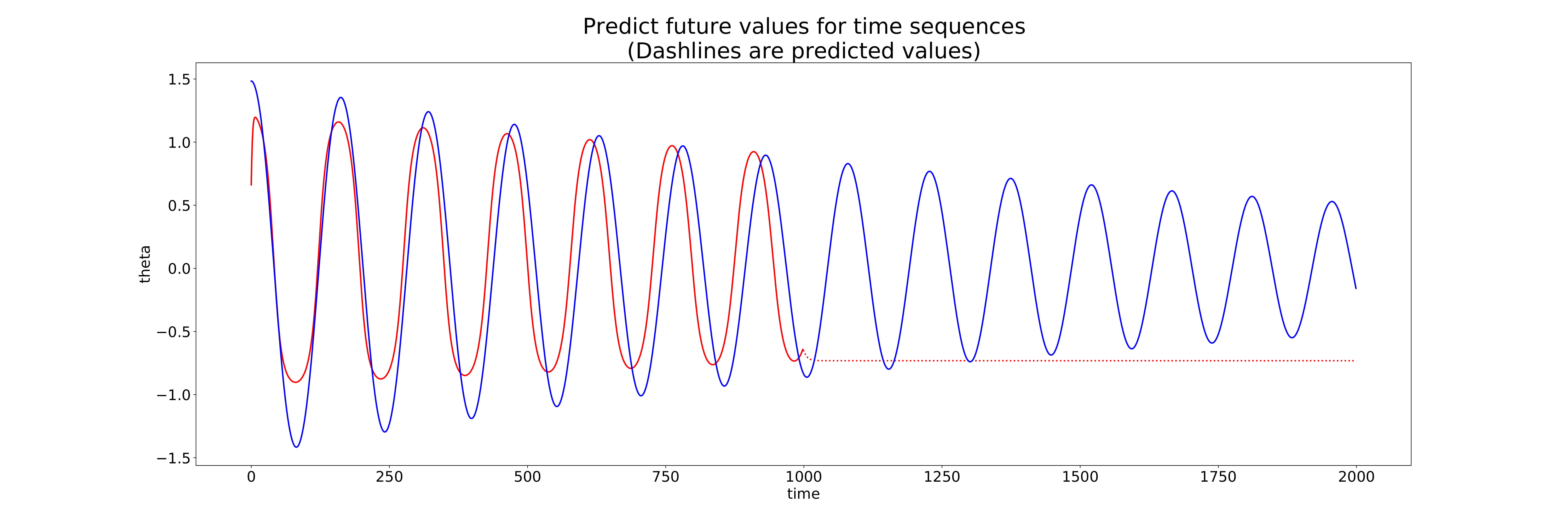
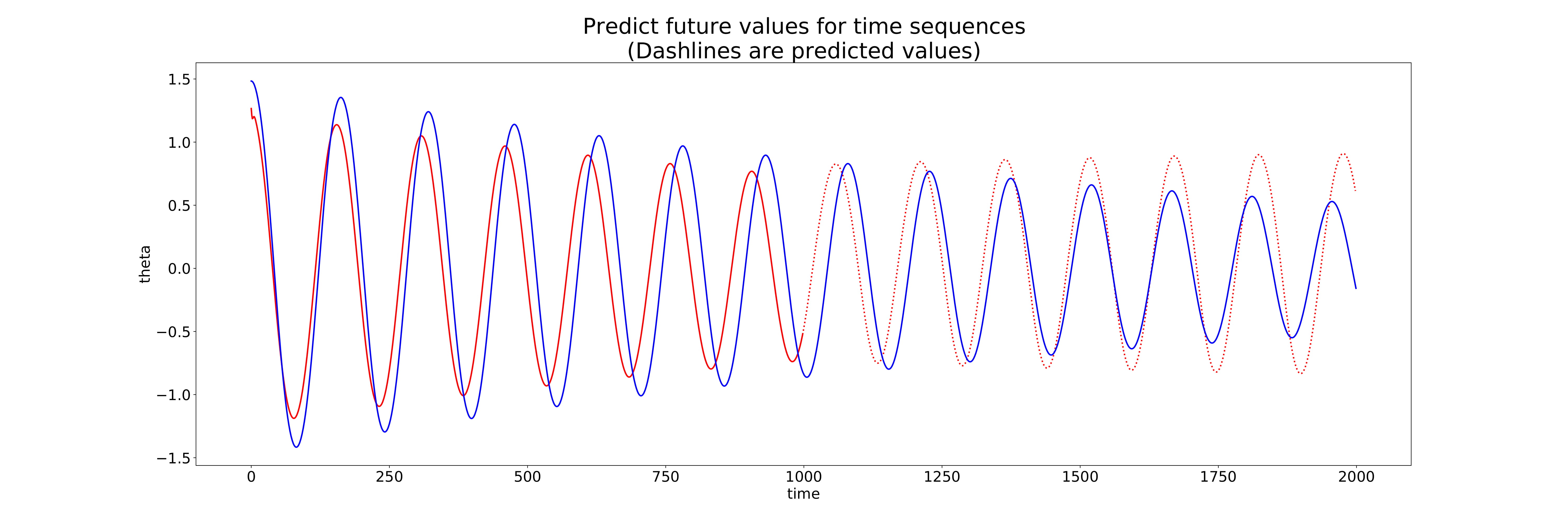
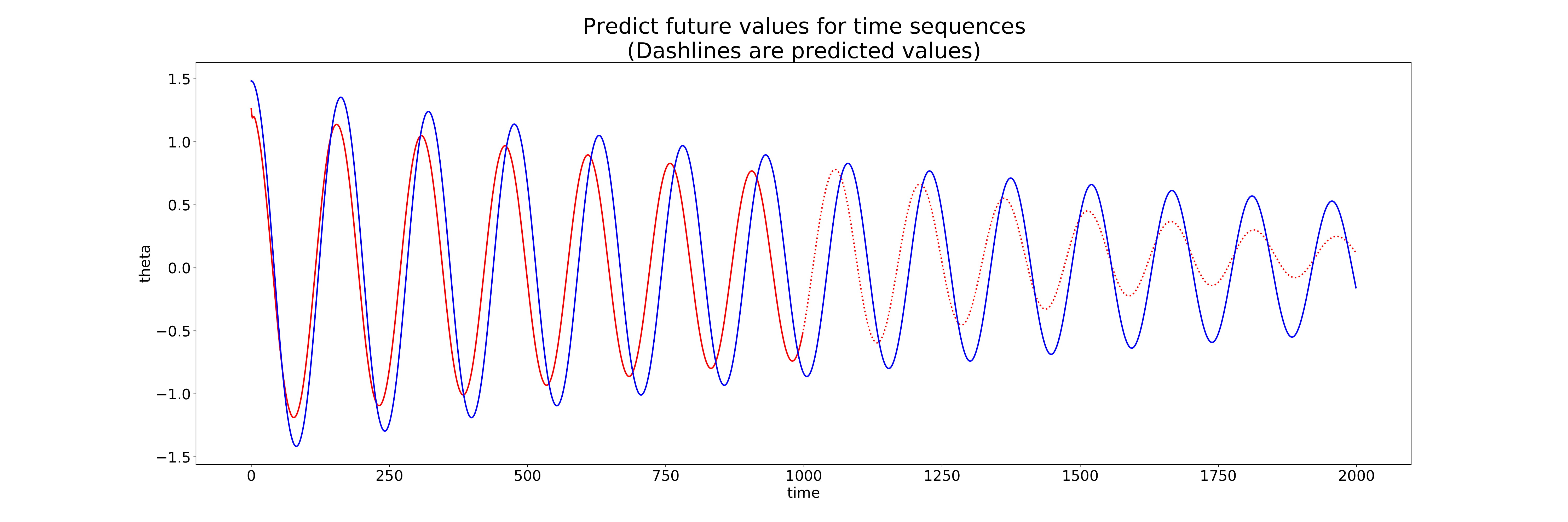
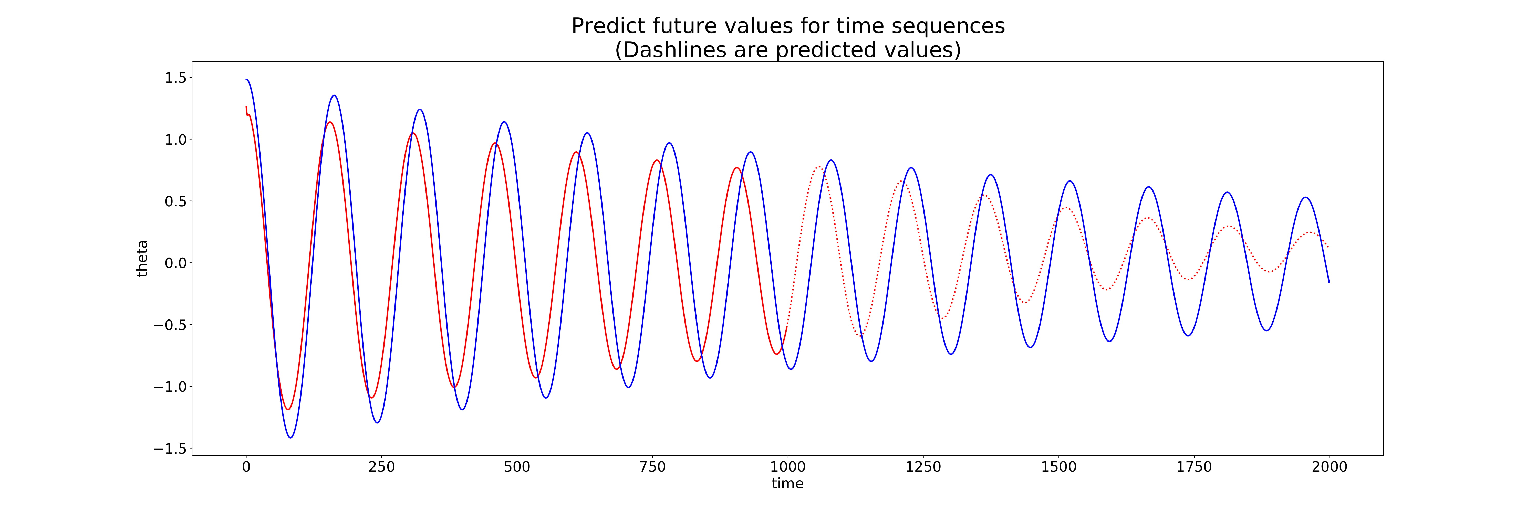
Below are the iteration results as the model trained. In the blue the actual solution for the pendulum problem, with the red solid line being the input to the model and the red dashed line being the predicted solution.
Prediction 1
Prediction 14
Prediction 54
Prediction 81
Prediction 100

As we can see, almost immediately on iteration 14, the model gets quite close to the actual solution, being further reduced as the iterations continue. We can see thought that on the final iteration, the model predicts in the ball park of the solution, but doesn’t reach the peaks and valleys of the solution. For a prediction, the RNN is quite conservative in magnitude of the prediction which I would say is better than an over-prediction.
Discussion
The RNN I constructed my not have accurately predicted the full path of a pendulum in 100 training iterations, however this was a fantastic learning experience for my first neural network project. There are still a lot of things I want to do with this though; I would like to train the model further past 100 iterations, I would like to add an adaptive learning rate for the optimizer to help converge on a solution faster, and I would like to have a wider training and prediction range for my pendulum solution. With this base I would love to continue my work, and will be updating this page with any improvements I make to the model!
.jpg)